The Pandas library, the best library for financial data

In the realm of finance, Excel is undeniably the go-to software. In this episode, we'll explore a library that allows us to accomplish everything Excel does, more and even better ! 📊

Introduction to Pandas

Pandas is a renowned Python library, boasting flexible data structures and efficient data analysis tools. It's especially tailored for financial data processing and is a favourite among financial analysts. Pandas runs on the NumPy platform, a cornerstone for scientific calculations in Python.

In this section, we'll delve into the essentials of Pandas, spanning from data creation and manipulation to its analysis.

Installing and Importing Pandas

With Pandas, we must introduce the concept of libraries in Python. Python's strength lies in its vast array of libraries, making development a breeze. Libraries are installed using the pip package manager that's bundled with Python installations.

To get started with Pandas, first, install it with the command:

pip install pandas

Once set up, import Pandas into your Python script with:

import pandas as pd

The alias "pd" is a standard convention in the Pandas community, offering a convenient shorthand for future use.

The DataFrame and Series Objects

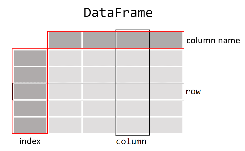
At the heart of Pandas are the DataFrame and Series objects. A DataFrame is a two-dimensional data array, resembling a database table or an Excel sheet. A Series, on the other hand, is a one-dimensional array, much like a list or a column in a DataFrame. Both have Indexes, which, if unspecified, default from 0 to the size of the data set, assigning an index to every row.

Here's a hands-on example:

import pandas as pd

data = {
    "date": ["2022-01-01", "2022-01-02", "2022-01-03", "2022-01-04"],
    "close": [150.0, 152.0, 153.0, 154.0],
    "volume": [1000, 1200, 1300, 1250],
}

df = pd.DataFrame(data)

print(df) # Displays the DataFrame
print(df.index) # Showcases the Indexes
print(df["close"]) # Reveals the "close" Series

In this instance, we've constructed a dictionary with three lists: date, close, and volume, each illustrating dates, closing prices, and transaction volumes respectively. We then utilize pd.DataFrame() to create a DataFrame from this data. The print statements show how we can engage with various parts of the DataFrame.

Manipulating and Analyzing Financial Data with Pandas

Pandas is laden with features that simplify data manipulation and analysis. Here's a quick rundown:

Selecting Rows or Columns

These snippets show how to cherry-pick columns, rows, or values:

close_column = df["close"]
print(close_column)

first_row = df.iloc[0]
print(first_row)

first_close = df.iloc[0]["close"]
print(first_close)

close_volume_columns = df[['volume', 'close']]
print(close_volume_columns)

To select rows based on a condition, you can use comparison operations on the DataFrame columns. For instance, to select all rows where the volume is greater than 1210:

best_volume_rows = df.loc[df['volume'] > 1210]
print(best_volume_rows)

Reading Data from CSV or Excel Files

Financial data are typically stored in CSV or Excel files. CSVs are tabulated data where entries are separated by commas or other delimiters. Pandas streamlines the process of reading these files into DataFrames:

You can access a day-by-day APPL stock price CSV file here: https://github.com/RobotTraders/Python_For_Finance/blob/main/APPL_1D.csv

To download, click the highlighted download icon (circled in red in the image below).

GitHub is a powerhouse for software development, enabling collaboration and version control. It's also the home for many open-source projects, including those by Crypto Robot (https://github.com/CryptoRobotFr) and Robot Traders.

The data follows the OHLCV format, which is standard for representing asset prices over specified periods (here, every 4 hours): Open, High, Low, Close, and Volume.

After downloading and placing the CSV in your directory, load it into a DataFrame:

df = pd.read_csv("APPL_1D.csv)
print(df)

In this case, we've read the file to store its content in the df variable, a process analogous to when we created our first DataFrame like this:

data = {
    "date": ["2022-01-01", "2022-01-02", "2022-01-03", "2022-01-04"],
    "close": [150.0, 152.0, 153.0, 154.0],
    "volume": [1000, 1200, 1300, 1250],
}

df = pd.DataFrame(data)

But in this situation, rather than manually specifying our data, it comes directly from a file.

Exploring and Manipulating Financial Data

Once you've stored your financial data in a Pandas DataFrame, you can easily explore and manipulate this data. For instance, you can compute descriptive statistics, and filter data based on certain conditions.

Exploring Financial Data

Initially, a best practice when working with a file is to quickly explore its data to ensure the quality of the information. In reality, your data will rarely be perfect and ready for analysis. More often than not, you'll need to "clean" your data. To swiftly inspect your data, you can use the describe() method.

df = pd.read_csv("APPL_1D.csv")
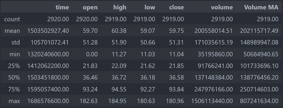
print(df.describe())

It's possible that your display shows scientific notations like e+03. This means, in this context, multiplication by 10 to the power of 3, or multiplication by 1000. Such notation becomes handy when dealing with very small or large numbers.

In our case, it hinders our analysis. So, you can insert the following line of code after importing pandas to round all numbers to two decimal places:

pd.set_option('display.float_format', lambda x: '%.2f' % x)

The describe() method provides several insights for each column. The count line indicates the number of entries. The lines labeled 25%, 50%, and 75% refer to quantiles, which we won't delve into here. The std line indicates the standard deviation. The other lines (mean, min, max) are self-explanatory.

By closely inspecting, we notice several issues in our data:

The presence of the Volume MA column, which we don't understand and seems irrelevant. The time and open columns have 2920 entries, while the others only have 2919. We need to find the row where other columns are missing values. The time column appears in a numeric format that we can't interpret. On closer observation, we see that the minimum of the open column is 0. It's unlikely that the opening price of APPLE was ever $0.

• To remove the Volume MA column:

  df = df.drop("Volume MA", axis=1)
  

• To find the missing values in the close column:

  print(df.loc[df["close"].isnull()])
  

Here, we see that the last row (with index 2919) contains values for the time and open columns but not for the others (NaN values mean “Not a Number”). This could be due to data being collected before the day ended, making the highest price, lowest price, volume, and closing price unavailable. To avoid complications later on, it's best to delete this row:

df = df.drop(2919)

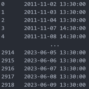
The time column contains very large numbers. After some research, we understand that these are dates in timestamp format. The numbers represent seconds elapsed since 1970. Fortunately, pandas has a method to convert these numbers to dates:

df["time"] = pd.to_datetime(df["time"], unit='s')
print(df["time"])

Now, with the dates being readable, we can replace our default indices (1, 2, 3…). Once that's done, we won't need our time column anymore and can delete it:

df = df.set_index(df['time'])
del df['time']

With our dates set as indices, it allows us to easily select one or multiple rows using date references:

print(df.loc["2023-05-04"]) # Displays the values for May 4, 2023
print(df.loc["2023-03"]) # Displays all the values for March 2023
print(df.loc["2023-03-03":"2023-03-15"]) # Displays the values from March 3 to March 15, 2023

Creating New Columns from Existing Ones

Pandas enables you to conveniently create new columns based on existing ones. For instance, you can make a column that represents the average of the opening and closing prices:

df["mean_open_close"] = (df["open"] + df["close"]) / 2
print(df["mean_open_close"])

What's crucial to understand here is that this operation is applied to all rows. You don't need to use a loop to apply this change to each row. Loops in Python can be time-consuming during execution, so it's beneficial to avoid them when possible.

Computing Descriptive Statistics

Pandas offers functions to compute descriptive statistics on your financial data. For instance, you can calculate the mean, median, standard deviation, and other statistics for stock prices of any company:

# Calculate descriptive statistics for each column
mean_prices = df["close"].mean()
median_prices = df["close"].median()
std_prices = df["close"].std()

print("Average closing prices:", mean_prices)
print("Median closing prices:", median_prices)
print("Standard deviation of closing prices:", std_prices)

Calculating a Moving Average

A moving average is a rolling price average. For example, the moving average value for a particular date would be the average of the prices for the previous 50 dates. To calculate rolling values with pandas, use rolling(50) followed by the operation you want to execute. For a 50-day moving average, you'd use rolling() followed by mean():

df["moving_average"] = df["close"].rolling(50).mean()

Calculating Returns and Volatility

After loading and prepping your data, you can conduct various financial analyses. For instance, you can calculate daily returns and the volatility of your asset. Volatility is a measure of the risk associated with an investment, typically calculated as the standard deviation of returns over a set period.

Here's an example of calculating daily returns and 30-day rolling volatility using Pandas:

# Calculate daily returns
df["daily_returns"] = df["close"].pct_change()

print(df["daily_returns"].head())

# Calculate 30-day rolling volatility
df["volatility"] = df["daily_returns"].rolling(window=30).std()

print(df["volatility"].head())

In this example, we use the pct_change() method to determine daily returns from stock prices. Then, we use the rolling() method to create a 30-day rolling window, followed by the std() method to determine the standard deviation (i.e., volatility) of returns over this rolling window.

Note that the first 29 rows of the volatility_30 column will have NaN (Not a Number) values, as there's not enough data to determine 30-day volatility for these rows. The head() method displays the first five rows.

Sorting Data

To sort data based on a column, you can use the sort_values() method on your DataFrame. For example, to sort data in ascending order by 30-day volatility:

df["daily_returns"] = df["close"].pct_change()
df["volatility"] = df["daily_returns"].rolling(window=30).std()
print(df.sort_values(by="volatility", ascending=True))
print(df.sort_values(by="daily_returns", ascending=True))

In this example, we first add 2 new columns to our DataFrame df. We then simply display our DataFrame df sorted from the lowest to highest volatility. Next, we display the days with the highest returns, from lowest to highest.

Mastering Your Data

Pandas is a comprehensive library, and we won't be able to explore all its features here.

It's essential to recognize that nearly any data manipulation is feasible with Python and the Pandas library. Your limits will be your technical skills and most importantly, your algorithmic capabilities. What we mean here is that the most significant challenge is often knowing precisely what you want to do, enabling you to search for the information online or in the official Pandas documentation. ChatGPT can be a valuable resource in this regard.

As we've previously highlighted, hands-on practice is the key. That's why we're presenting a practical exercise to reinforce your learning. But remember, practicing with your own data or problems is even better.

Application Exercise: The Titanic

For this exercise, we'll analyze data related to the Titanic's tragic voyage. You can find a CSV file representing each of the Titanic passengers, including their names, genders, classes (Pclass), ages, and other information here: https://github.com/RobotTraders/Python_For_Finance/blob/main/TITANIC.csv.

Instructions

Start by downloading the CSV file. Place it in your project directory, import Pandas, and load the CSV into a DataFrame:

df = pd.read_csv('TITANIC.csv')

Please note, for this exercise, you might need methods we haven't discussed yet, like value_counts() or groupby(). The goal is for you to conduct independent research.

Questions

1. Display the dataset's first ten rows to get an overview.
2. Determine the dataset's dimensions (i.e. the number of rows and columns).
3. Count the number of passengers in each class (Pclass).
4. Calculate the average age of passengers. Identify the youngest and oldest passengers by name.
5. Determine how many passengers survived and how many perished.
6. Count the number of male and female passengers aboard the Titanic.
7. How many men and women survived?
8. What's the survival rate by class?
9. Add a new 'FamilySize' column that sums the 'SibSp' (number of siblings/spouses aboard) and 'Parch' (number of parents/children aboard) columns.
10. Identify the non-survivor with the most significant family on board.

A correction example can be found here: https://github.com/RobotTraders/Python_For_Finance/blob/main/exercise_correction_chapter_5.ipynb